![The figure to the left [Simpson et al., 1992] is a cross section through one of the telescope devices](/media/migration/research-groups/Anisotropic-Telescope-Section--tojpeg_1448285043839_x2.jpg) The two Anisotropy Telescopes are identical solid state particle detectors with 70° opening angles and geometric factors of 0.7 cm2 sr. The figure to the right [Simpson et al., 1992] is a cross section through one of the telescope devices. Depending on the outputs of the the three detectors A,B and C, ions incident on the telescope will register a count in one of 13 data channels (see below for more information).
The two Anisotropy Telescopes are identical solid state particle detectors with 70° opening angles and geometric factors of 0.7 cm2 sr. The figure to the right [Simpson et al., 1992] is a cross section through one of the telescope devices. Depending on the outputs of the the three detectors A,B and C, ions incident on the telescope will register a count in one of 13 data channels (see below for more information).
Different channels are sensitive to ions of different energies such that the ATs system is capable of measuring protons in the energy range 0.7-6.7 MeV. Helium, oxygen and sulphur nuclei can also be detected in some data channels but the instrument does not distinguish counts according to ion species.
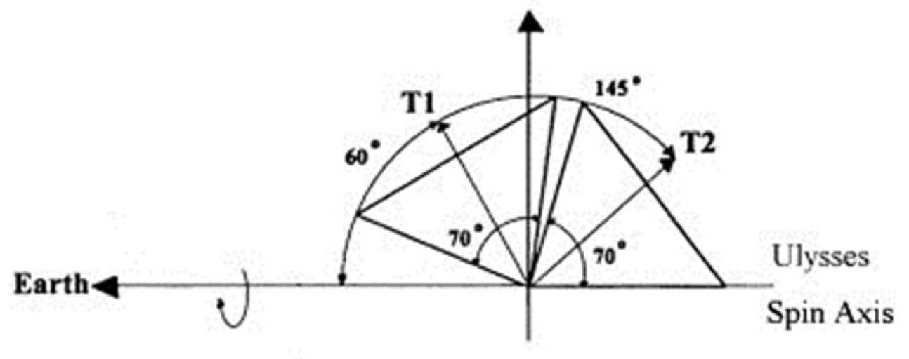
The figure below shows a schematic view of the ATs instrument. The two telescopes (T1 & T2) are mounted on the spacecraft at the angles shown giving excellent angular coverage. Each time Ulysses spins about the axis shown, the counts detected in some channels are separated into eight 45° sectors. This means that each sector corresponds to a particular viewing direction with a total of 16 viewing or look directions provided by the two telescope system.
 From these measurements we attempt to calculate if there is a directional dependence in the ion fluxes calculated from the count rates. If the ion flux is the same in all directions the ion distribution is isotropic, but, as the instrument name suggests, if the flux is larger in one direction than the others the ion distribution is anisotropic. The anisotropic nature of the fluxes helps us understand the underlying physics of space plasma media.
There is information on how these calcuations are done in the calculate the anisotropy section below.
ATs Instrument Description
If the number of ion counts in the energy channel we are interested is sufficiently high to be unaffected by Poisson statistics [i.e. 1/root(no. of counts)] then we deduce the anisotropy present in the ion flux distribution in the following way. The ion counts are converted into fluxes and then we use the 16 measurements from the 2 telescope 8 sector system to make a spherical harmonic fit to the flux distribution using the equation below.
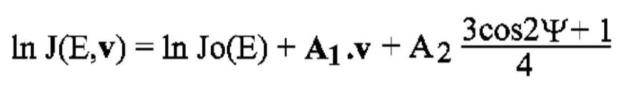
Where J is the differential flux, Jo the omnidirectional flux, E the ion energy, v the ion unit velocity vector, A1 the first order anisotropy vector, A2 the second order anisotropy magnitude and psi the particle pitch angle.
The fit above yields the first order anisotropy vector which can be resolved into field aligned and field perpendicular components. Field perpendicular components can arise either due to a bulk flow of the plasma or due to a spatial gradient in the ion flux, or as a combination of the two effects. Anisotropies parallel to the magnetic field need not be simply related to the thermal flow of the plasma and generally pertain to the nature of the ions from which they were derived. The parallel anisotropy component tells us about the asymmetry of the particle distribution in the bulk flow frame.
The ATs report back ion counts which are stored in 13 different data channels. The channels vary both in energy sensitivity and temporal resolution. Some channels report spin averaged data whilst others report sectored data. The table below summarises each channel's characteristics. The sectored channels are highlighted in bold.
| Channel No. | Energy Range (MeV) | No. of Sectors | Best Time Resolution (s) | |||
| Protons | Alphas | Oxygen | Sulphur | |||
| 1 2 3 4 5 6 7 8 9 10 11 12 13 |
0.7-0.9 0.9-1.3 1.3-2.2 2.2-3.6 3.6-6.7 0.7-1.3 1.3-2.2 2.2-3.6 3.6-6.7 - - - - |
2.3-2.5 2.5-2.7 2.7-3.0 - 24-28 2.3-2.7 2.7-3.0 - 24-28 3.0-7.5 7.5-12.0 12-26 3.0-7.5 |
20.5-21.5 21.5-22.5 22.5-23.5 - - 20.5-22.5 22.5-23.5 - - 23.5-63.0 63-65 65-240 23.5-63 |
63-65 65-67 67-69 - - 63-67 67-69 - - 69-185 185-210 210-750 69-185 |
Spin-averaged Spin-averaged Spin-averaged Spin-averaged Spin-averaged 8 8 8 8 Spin-averaged Spin-averaged Spin-averaged 4 |
16 16 16 16 16 16 64 64 64 128 128 128 128 |
Notice that we may use channels 6 through 9 for anisotropy analysis. In the solar wind we exploit channel 7 data first since it is least affected by background problems but still has reasonably high fluxes to avoid counting statistics errors. At Jupiter we have used both channel 6 and channel 7 anisotropy data.